
Why We Divide by ( n-1 ) When Calculating Sample Variance
If you’ve ever worked with statistics, you’ve probably seen this little quirk in the formula for variance:
\[s^2 = \frac{\sum (x_i - \bar{x})^2}{n - 1}\]Why ( n - 1 ) instead of just ( n )?
It’s not a random tradition it’s a mathematical correction that makes your estimate unbiased. In this post, I’ll show you two experiments that make the idea visually clear:
a. one with a normally distributed population, and

b. one with a non-normal (uniform) population,

c. plus the intuitive theory behind it.
Experiment 1: Normally Distributed Population
Setup:
- Population: Normally distributed with mean = 50, std = 10, size = 50,000.
- True variance calculated directly from the population.
- Sample sizes: 10 to 100.
- Variance estimated using different divisors:
- Each sample size repeated 500 times, and results averaged.
Result:
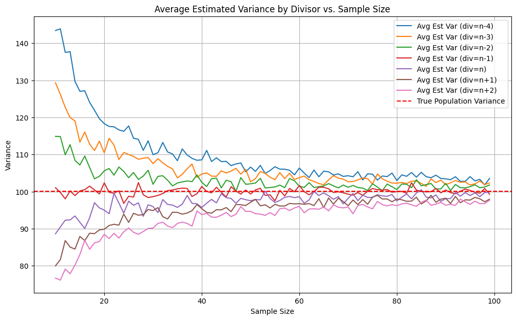
The red dashed line is the true variance.
The red solid line (dividing by (n-1)) sticks closest to the truth across all sample sizes.
Dividing by (n) underestimates variance; using (n-2) or smaller overestimates it.
If you want to run the code and play around with the sample size/population/repetitions etc the code and data used to generate the graph above can be found here.
View the Jupyter notebook code here
Experiment 2: Uniform Population
One might wonder…. what if the population isn’t normal? Does the (n-1) correction still hold?
To check, I repeated the experiment with a population consisting of the integers 1 to 50,000.
Result:
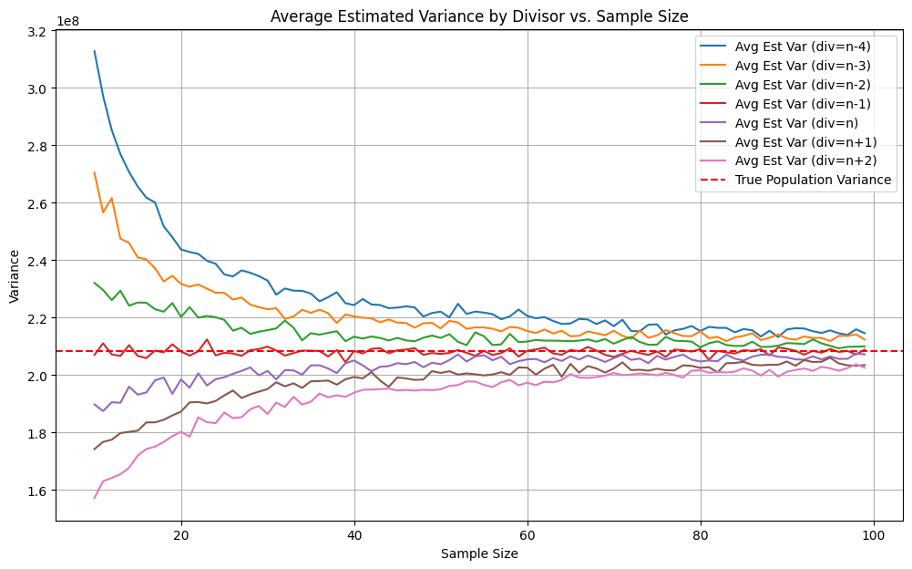
The pattern is the same:
- (n-1) still gives the best unbiased estimate of the true variance.
- Bias from using (n) or other divisors is visible, especially at smaller sample sizes.
This tells us that Bessel’s correction works regardless of whether the underlying population is normal, uniform, or otherwise. It’s a property of sampling, not of the distribution shape.
If you want to run the code and play around with the sample size/population/repetitions etc the code and data used to generate the graph above can be found here.
View the Jupyter notebook code here
Why ( n - 1 ) Works: The Theory
When calculating sample variance, we use the sample mean ($\bar{x}$) in place of the true population mean ($\mu$).
This introduces a bias because:
- The deviations from ($\bar{x}$) are, on average, smaller than deviations from ($\mu$).
- That’s because ($\bar{x}$) is calculated from the sample itself and “pulls” towards the data points.
To correct for this, we divide by (n - 1) instead of (n). This is called Bessel’s correction, and it ensures that the expected value of the sample variance equals the true variance.
A Simple Intuition: Degrees of Freedom
Imagine you have just two numbers in your sample.
Once you know the mean, the second number’s deviation is completely determined by the first, there’s no extra “freedom” left. You’ve lost one degree of freedom.
In general:
- When estimating the variance, one degree of freedom is used up in estimating the mean.
- That’s why you divide by (n - 1) instead of (n).